Unleashing the Power of Big Data Analysis with Power Query and Power Pivot in Excel

By Gustiyan Islahuzaman

Introduction

In the era of information explosion, businesses are grappling with colossal amounts of data. The ability to harness this data and derive meaningful insights has become a crucial competitive advantage. Enter Power Query and Power Pivot, two powerful tools within Microsoft Excel that empower users to efficiently manage, transform, and analyze big data. In this article, we’ll explore the prowess of Power Query and Power Pivot in unraveling the potential of big data analysis.

To illustrate the capabilities of Power Query and Power Pivot in Excel, let’s dive into an example analysis using sales data. Imagine you have a massive sales dataset with a total of 1,624,039 rows, stored in a TXT format. The data is separated into files for the years 2015, 2016, and 2017. Our goal is to perform data analysis on this dataset and create an interactive dashboard for insights.

Prerequisites for Harnessing Power Query and Power Pivot

Before embarking on your journey to analyze big data using Power Query and Power Pivot in Excel, it’s essential to ensure that you have the necessary prerequisites in place. These prerequisites will enable you to fully unleash the potential of these powerful tools and make the most of your data analysis efforts.

1. Microsoft Excel Version: Excel 2016 or Later

To utilize Power Query and Power Pivot, you need a minimum version of Microsoft Excel 2016. These features are integrated into Excel starting from this version, and subsequent updates have introduced improvements and new functionalities. Using the latest version of Excel is recommended to benefit from the most up-to-date capabilities.

2. Activating Power Pivot Add-In

While Excel 2016 and later versions include Power Pivot, it might not be activated by default. To enable Power Pivot, follow these steps:

1. Go to the “File” tab in Excel.
2. Click on “Options” at the bottom of the left-hand menu.
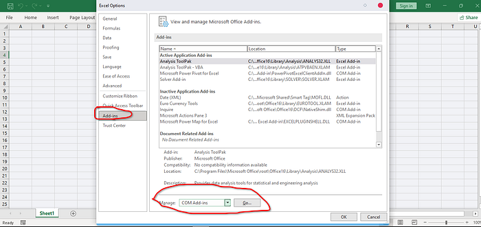
3. In the Excel Options window, select “Add-Ins” from the left sidebar.
4. In the “Manage” dropdown at the bottom, choose “COM Add-ins” and click “Go…”
5. Check the “Microsoft Office Power Pivot” option and click “OK.”
6. This will activate the Power Pivot add-in, and you’ll find the “Power Pivot” tab added to the Excel ribbon.

Step 1: Importing Data with Power Query

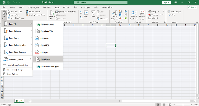
1. Open Excel and go to the “Data” tab.
2. Click on “Get Data” and select “From Folder” to import the sales data from the TXT files for each year.
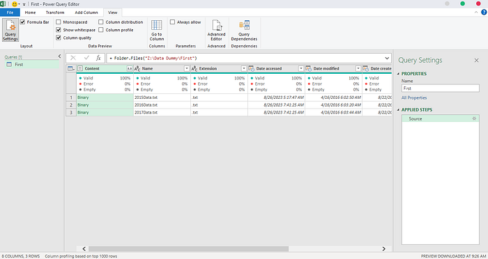
3. In the Power Query Editor, you can perform various data transformations using Power Query’s intuitive interface. Cleanse, transform, and shape the data as needed. This might include removing unnecessary columns, handling missing values, and converting data types.

Step 2: Merging Data with Power Query

1. Since the sales data is separated into files for different years, you can use Power Query to merge the data into a single table.
2. Add a custom column to each dataset to indicate the year, and then append the datasets together.

Step 3: Creating Relationships and Data Model with Power Pivot

1. Once you’ve prepared your data, go to the “Power Pivot” tab and click on “Add to Data Model” to create a data model.
2. Define relationships between tables based on common fields, such as customer IDs and product IDs.
3. Create calculated columns and measures using DAX language. For instance, you can calculate total sales, average order value, and year-over-year growth.

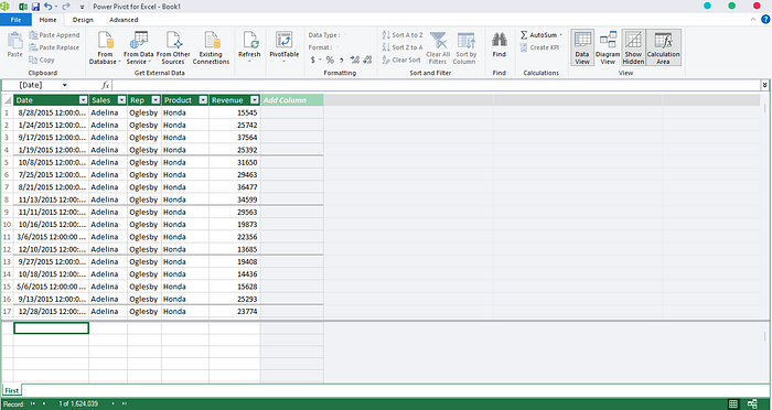
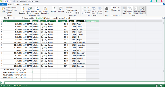
Step 4: Building an Interactive Dashboard

1. Go back to your Excel workbook and insert a new worksheet for the dashboard.
2. Utilize PivotTables and PivotCharts to visualize your data. For example, create a PivotChart that displays total sales over the years.
3. Add slicers for filtering data by year, region, or product category. Slicers provide an interactive way to explore your data dynamically.
4. Create a PivotTable with a calculated field showing the top products or customers based on specific metrics.

Step 5: Sharing and Updating the Dashboard

1. Once you’ve built your interactive dashboard, you can save and share the Excel file with colleagues or stakeholders.
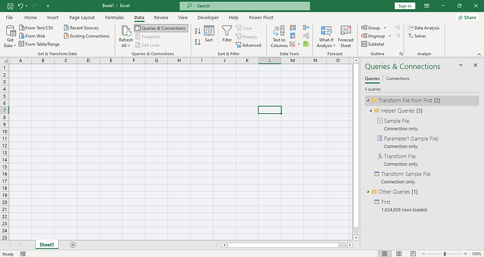
2. When you receive new sales data for subsequent years, you can easily update the dataset by refreshing the data connections in Power Query.
3. The Power Pivot data model will automatically update, and your dashboard will reflect the latest insights.

Conclusion

In this example analysis, we’ve demonstrated how to utilize Power Query and Power Pivot to transform raw sales data into a powerful analytical tool. By integrating data from multiple sources, performing transformations, and creating relationships, you can build a comprehensive data model. The interactive dashboard, enriched with PivotTables, PivotCharts, and Power View visualizations, empowers you to explore data, identify trends, and make data-driven decisions.

The synergy between Power Query’s data preparation capabilities and Power Pivot’s advanced analysis features showcases Excel’s potential for big data analysis. This example serves as a testament to the effectiveness of these tools in handling large datasets and creating actionable insights, proving that Excel remains a valuable tool for data professionals in the era of big data.