Mastering Imbalanced Classification: XGBoost and SMOTE + ENN on Bank Marketing Data With Python

by Gustiyan Islahuzaman

10 min readAug 29, 2023

Introduction

In the realm of machine learning, classification stands as a cornerstone, allowing us to predict class labels based on input features. However, the challenge of imbalanced datasets, characterized by skewed class distributions, often emerges. In this article, we delve into overcoming this challenge through the synergistic collaboration of XGBoost and the SMOTE + ENN algorithm. Together, they present a potent solution that reshapes predictions within the context of the Bank Marketing dataset. To explore this journey in its entirety, you can access the full notebook on my Google Colab (link). Additionally, for a more immersive understanding of this topic, I invite you to watch my presentation about this article here.

Dataset Analysis and Overview

Before embarking on our classification journey, let’s delve into the foundation of data integrity. Sourced from Kaggle, our dataset is a realm of insights, comprising 21 columns and an impressive 41,188 rows.
Attribute Information: Within this landscape, we explore a rich tapestry:

1. Input Variables:

Age: Numeric age of the client.
Job: Categorical occupation.
Marital Status: Categorical marital status.
Education: Educational level, a categorical feature.
Default: Credit default status (categorical).
Housing: Housing loan status (categorical).
Loan: Personal loan status (categorical).
Contact: Method of contact (categorical).
Month: Month of the last contact (categorical).
Day of Week: Day of the week of the last contact (categorical).
Duration: Duration of the last contact in seconds (numeric).
Campaign: Number of contacts during this campaign for the client (numeric).
Days Since Previous Contact: Days since the client’s last contact from a previous campaign (numeric; 999 denotes no previous contact).
Previous Contacts: Number of contacts before this campaign for the client (numeric).
Previous Campaign Outcome: Outcome of the previous marketing campaign (categorical).
Employment Variation Rate: Quarterly employment variation rate (numeric).
Consumer Price Index: Monthly consumer price index (numeric).
Consumer Confidence Index: Monthly consumer confidence index (numeric).
Euribor 3-Month Rate: Daily Euribor 3-month interest rate (numeric).
Number of Employees: Quarterly number of employees (numeric).

Output Variable (Target):

Subscription: Binary indicator of whether the client subscribed to a term deposit (“yes” or “no”).

Our voyage begins by sculpting data quality and embracing its nuances. As we traverse this domain, the marriage of numbers, categories, and trends shall guide our classification odyssey. Let’s delve further, where insight and analysis converge in pursuit of precision.

Data Preprocessing and Set-Up

Cleaning Data: Before diving into analysis, we tidy up our dataset. This involves spotting and fixing errors, handling missing values, and ensuring data consistency.

Standardizing Data: Next, we bring uniformity to our data. Standardization adjusts values to a common scale, aiding fair comparison across features.

Encoding Data: To bridge the gap between words and numbers, we employ encoding. This translates categorical data into numerical form, ready for analysis.

With these simple yet powerful steps, we lay the groundwork for extracting insights and patterns from our data. Setting Up the Workspace: Our journey starts with assembling the essential tools. We’ve enlisted the aid of well-loved Python libraries:

sklearn: Packed with machine learning methods and performance metrics.
pandas: Facilitates smooth handling of structured data.
numpy: The trusted companion for numerical operations.
matplotlib: Our versatile ally for crafting visualizations.
seaborn: Elevates our visual storytelling with statistical graphics.
xgboost: Our knight in shining armor for creating powerful predictive models.

Together, these tools empower us to embark on an insightful exploration, unveiling the hidden stories within our data.

Cleaning Data: Streamlining for Analysis

Loading Data: Our journey commences with loading the dataset. We bring it into our workspace, preparing to unveil its hidden stories.

# Import libraries
import xgboost as xgb
import pandas as pd
import numpy as np
import matplotlib.pyplot as plt
import seaborn as sns
from sklearn.model_selection import train_test_split
from sklearn.metrics import accuracy_score, classification_report
import warnings
# Suppress all warnings
warnings.filterwarnings('ignore')
# Load dataset
data_path = 'https://raw.githubusercontent.com/gustiyaniz/
↪PwCAssigmentClassification/main/bank-additional-full.csv'
df = pd.read_csv(data_path,sep=";",header=0)
# print(df info())
print('Shape of dataframe:', df.shape)
df.head()

2. Checking Data Types: Understanding data is crucial. We examine the data types of various columns to ensure they align with their content. This step paves the way for accurate analysis.

from sklearn.preprocessing import StandardScaler
#names columns
columns = list(df.columns)
columns
# check datatype in each column
print("Column datatypes: ")
print(df.dtypes)
# Copying original dataframe
df_set = df.copy()

3. Removing Unnecessary Columns: Not all columns contribute equally. We streamline our dataset by removing irrelevant columns, such as ‘duration’, to focus on what truly matters.

# Drop 'duration' column
df = df.drop(columns='duration')
df.head()

With this streamlined approach, we ensure our dataset is primed for meaningful analysis, setting the stage for insightful discoveries.

Standardizing Data
To standardize the numerical columns in our dataset, we’ll use the StandardScaler from the sklearn.preprocessing module. This scaler will transform our data to have a mean of 0 and a standard deviation of 1.

from sklearn.preprocessing import StandardScaler
#names columns
columns = list(df.columns)
columns
# check datatype in each column
print("Column datatypes: ")
print(df.dtypes)
# Copying original dataframe
df_set = df.copy()
#standarization data numeric
scaler = StandardScaler()
num_cols = ['age', 'campaign', 'pdays', 'previous','emp.var.rate',
'cons.price.idx','cons.conf.idx','euribor3m','nr.employed']
df_set[num_cols] = scaler.fit_transform(df[num_cols])
df_set.head()

Encoding Data: Transforming with OneHotEncoder
OneHotEncoder is a nifty tool that takes categorical data (like ‘red’, ‘green’, ‘blue’) and transforms it into a numerical format that computers can understand. It creates separate columns for each category, assigning 1 or 0 to indicate the presence or absence of that category in a particular row, making data suitable for analysis and modeling.

#Encoding Categorical Data To Format Numeric
from sklearn.preprocessing import OneHotEncoder

# Create the encoder and categorical columns
encoder = OneHotEncoder(sparse=False)
cat_cols = ['job', 'marital', 'education', 'default', 'housing', 'loan', 
            'contact', 'month','day_of_week','poutcome']

# Encode Categorical Data
df_encoded = pd.DataFrame(encoder.fit_transform(df_set[cat_cols]))
df_encoded.columns = encoder.get_feature_names_out(cat_cols)

# Drop Categorical Data and Concatenate Encoded Data
df_set = df_set.drop(cat_cols, axis=1)
df_set = pd.concat([df_encoded, df_set], axis=1)

# Encode target value
df_set['y'] = df_set['y'].apply(lambda x: 1 if x == 'yes' else 0)

# Print the shape and the first few rows of the DataFrame
print('Shape of dataframe:', df_set.shape)
df_set.head()

Data Analysis: Unveiling Patterns and Enhancing Predictions

Oversampling with SMOTE-ENN Algorithm
Diving into analysis, we tackle the challenge of imbalanced data with the SMOTE-ENN algorithm. This dynamic duo creates balance by generating synthetic samples for the minority class and cleaning noisy data, improving our model’s accuracy.

#Split Dataset for Training and Testing
# Select Features
feature = df_set.drop('y',axis=1) # Features (input variables)

# Select Target
target = df_set['y'] # Target (output variable)

# Set Training and Testing Data
from sklearn.model_selection import train_test_split
X_train, X_test, y_train, y_test = train_test_split(feature , target,
                                                    shuffle = True,
                                                    test_size=0.2,
                                                    random_state=1)
#sampling imbalance class with smoth + enn algorithm
from imblearn.combine import SMOTEENN
import collections
counter = collections.Counter(y_train)
print('Before', counter)
# oversampling the train dataset using SMOTE + ENN
smenn = SMOTEENN()
X_train_smenn, y_train_smenn = smenn.fit_resample (X_train, y_train)
counter = collections.Counter (y_train_smenn)
print('After', counter)

2. XGBoost Classification
Enter XGBoost, a powerhouse in classification. We harness its might to create a classification model that learns from the data’s intricate patterns, making accurate predictions.

from sklearn.metrics import accuracy_score, cohen_kappa_score, f1_score, recall_score, precision_score, confusion_matrix

# Initialize and train the XGBoost classifier
xgb_classifier = xgb.XGBClassifier(n_estimators=100, max_depth=3, n_jobs=-1, learning_rate=0.5, random_state=42)
xgb_classifier.fit(X_train_smenn, y_train_smenn)

# Make predictions using the model
y_pred = xgb_classifier.predict(X_test)

# Calculate evaluation metrics
accuracy = accuracy_score(y_test, y_pred)
kappa = cohen_kappa_score(y_test, y_pred)
f1 = f1_score(y_test, y_pred)
recall = recall_score(y_test, y_pred)
precision = precision_score(y_test, y_pred)

# Print the evaluation metrics
print("Results With Oversampling Smote + ENN")
print("XGBoost Accuracy:", accuracy)
print("Kappa Score:", kappa)
print("F1 Score:", f1)
print("Recall:", recall)
print("Precision:", precision)

#print confusion matrix
cm = confusion_matrix(y_test, y_pred)

# Create a heatmap for the confusion matrix
plt.figure(figsize=(8, 6))
sns.set_theme(style="whitegrid")
sns.heatmap(cm, annot=True, fmt="d", cmap="Blues", cbar=False)
plt.title('Confusion Matrix - XGBoost with SMOTE')
plt.xlabel('Predicted')
plt.ylabel('Actual')
plt.show()

3. Comparing XGBoost with SMOTE and Without
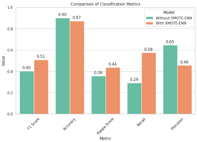
We don our detective hats and compare XGBoost’s performance with and without SMOTE. By observing accuracy, precision, recall, and F1-score, we gauge the tangible impact of balancing our dataset on classification outcomes.

# Create a DataFrame for visualization
metrics = ['F1 Score', 'Accuracy', 'Kappa Score', 'Recall', 'Precision']
values_nosmote = [f1_nosmote,
                  accuracy_nosmote,
                  kappa_nosmote,
                  recall_nosmote,
                  precision_nosmote]

values_smote = [f1,
                accuracy,
                kappa,
                recall,
                precision]

# Create a DataFrame for visualization
data = {
    'Metric': metrics * 2,
    'Model': ['Without SMOTE-ENN'] * len(metrics) + ['With SMOTE-ENN'] * 
            len(metrics),
    'Value': values_nosmote + values_smote
}
metrics_df = pd.DataFrame(data)

# Create a bar plot using Seaborn
plt.figure(figsize=(10, 6))
sns.set_theme(style="whitegrid")
ax = sns.barplot(x='Metric', y='Value', hue='Model', data=metrics_df, 
                  palette="Set2")
plt.title('Comparison of Classification Metrics')
plt.xticks(rotation=45)
plt.ylim(0, 1)  # Adjust the y-axis range if needed
plt.legend(title='Model', loc='upper right')

# Annotate bars with values
for p in ax.patches:
    ax.annotate(format(p.get_height(), '.2f'),
                (p.get_x() + p.get_width() / 2., p.get_height()),
                ha='center', va='center',
                xytext=(0, 10),
                textcoords='offset points')

plt.show()

Observations:

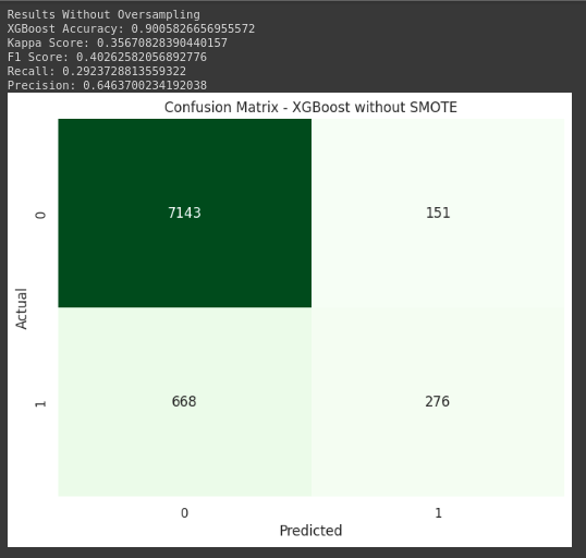
The model XGBoost without Oversampling achieved a higher accuracy (0.9006) compared to the model XGBoost with SMOTE + ENN (0.8725). However, the Kappa Score, which considers the agreement between observed and expected outcomes, is higher for the model with oversampling (0.4363 vs. 0.3567). This suggests that the improvement in accuracy for the model without oversampling might be partially attributed to the class imbalance.
The F1 Score and Precision are both higher for the model with oversampling (0.5084 and 0.4555, respectively) compared to the model without oversampling (0.4026 and 0.6464, respectively). This indicates that the model with oversampling performs better at achieving a balance between precision and recall, especially in the context of imbalanced data.
The Recall, also known as sensitivity or true positive rate, is significantly higher for the model with oversampling (0.5752) compared to the model without oversampling (0.2924). This means the model with oversampling is better at correctly identifying instances of the minority class.

Feature Importance Analysis

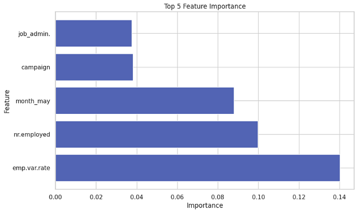
As the XGBoost model is being trained, it assigns importance scores to each feature based on how much they contribute to reducing the model’s prediction error. Features that help the model make accurate predictions are assigned higher importance scores, while less influential features receive lower scores.

# Get feature importances
feature_importances = xgb_classifier.feature_importances_

# Create a DataFrame to store feature importances
feature_importance_df = pd.DataFrame({'Feature': X_train.columns, 'Importance': feature_importances})

# Sort features by importance
feature_importance_df = feature_importance_df.sort_values(by='Importance', ascending=False)

# Select the top 5 most important features
top_features = feature_importance_df.head(5)

# Plot feature importances for the top 5 features
plt.figure(figsize=(10, 6))
plt.barh(top_features['Feature'], top_features['Importance'])
plt.xlabel('Importance')
plt.ylabel('Feature')
plt.title('Top 5 Feature Importance')
plt.show()

In this feature analysis using the XGBoost algorithm, we have gained valuable insights into the variables that play a significant role in predicting our target variable. Among the analyzed features, the “Employment variation rate” has emerged as the most influential variable, with the highest importance score. This suggests that changes in the employment variation rate have a substantial impact on our predictions.

Additionally, the top 5 influential variables include:

Number of Employees: The “Number of employees” variable has shown a strong influence on our prediction outcomes. The quantity of employees associated with a scenario significantly affects the result.
Job Administration: The presence or absence of the “job admin” role is a key predictor, suggesting its importance in determining the prediction outcome.
Marital Status “Single”: The marital status of “single” has proven to be a significant factor in making accurate predictions. It significantly contributes to the predicted outcome.
Month of May: The month of May has surfaced as an important time period affecting predictions. This could indicate a seasonality or pattern linked with May that impacts the outcome.

These findings provide valuable insights for refining our predictive models and making informed decisions based on the predictions. It’s important to validate these insights in the context of the domain and continuously monitor their relevance.

Output and Saving Variables: Preserving Insights

Adding Prediction Labels to the Dataset: Our journey comes full circle as we enrich the dataset with prediction labels. This addition showcases how our model classifies each instance, offering a holistic view of the classification outcomes.

import joblib

# Make predictions for the entire dataset
all_predictions = xgb_classifier.predict(feature)

# Convert 1 to 'yes' and 0 to 'no'
all_predictions = ['yes' if pred == 1 else 'no' for pred in all_predictions]

# Add predictions to the original dataset
df['Predicted_Labels'] = all_predictions

# Save the augmented dataset
df.to_csv('augmented_dataset.csv', index=False)

# Results Without Oversampling
results_nosmote = {
    'Model': 'XGBoost without Oversampling',
    'Accuracy': accuracy_nosmote,
    'Kappa Score': kappa_nosmote,
    'F1 Score': f1_nosmote,
    'Recall': recall_nosmote,
    'Precision': precision_nosmote
}

# Results With Oversampling (SMOTE + ENN)
results_smote = {
    'Model': 'XGBoost with SMOTE + ENN',
    'Accuracy': accuracy,
    'Kappa Score': kappa,
    'F1 Score': f1,
    'Recall': recall,
    'Precision': precision
}

2. Saving the XGBoost Model: Our analysis yields a robust XGBoost model. We don’t want to lose this gem! We save the model to be used in the future, ensuring we retain its predictive prowess.

# Save results using joblib
joblib.dump(results_nosmote, 'results_nosmote.pkl')
joblib.dump(results_smote, 'results_smote.pkl')
joblib.dump(xgb_classifier, 'xgb_classifier_smote.pkl')
joblib.dump(xgb_classifier_nosmote, 'xgb_classifier_nosmote.pkl')

# Load saved results
loaded_results_nosmote = joblib.load('results_nosmote.pkl')
loaded_results_smote = joblib.load('results_smote.pkl')
loaded_xgb_classifier_smote = joblib.load('xgb_classifier_smote.pkl')

print("Loaded Results Without Oversampling:", loaded_results_nosmote)
print("Loaded Results With Oversampling (SMOTE + ENN):", loaded_results_smote)
print("Loaded XGBoost Classifier Model",loaded_xgb_classifier_smote)

As we conclude this phase, we not only preserve our hard-earned results but also imbue our dataset with newfound knowledge, making it a richer resource for future insights.

Conclusion

In closing, the dynamic blend of XGBoost classification and the SMOTE + ENN algorithm stands as a robust approach for handling imbalanced datasets. Our journey underscores the significance of preprocessing and balanced class distributions in achieving accurate classification outcomes. By preserving these findings, we enhance our dataset for future explorations and analyses, enabling the creation of a predictive model for bank subscription. Moreover, we’ve pinpointed the top 5 influential features that impact subscription outcomes, empowering us with valuable insights into customer behaviors and preferences.

References