House Price Prediction With XGBoost Using R Markdown

Introduction
In the ever-evolving world of real estate, knowing how to predict house prices is a valuable skill. Whether you are a homeowner looking to estimate the value of your property or a real estate professional trying to make informed decisions, machine learning can be a powerful tool to make accurate predictions. In this article, we will explore how to create a house price prediction model using XGBoost, a popular gradient boosting algorithm, in R. We will also leverage R Markdown to document our analysis and share it effectively. If you’d like to see the R Markdown code and analysis in action, you can view my complete R Markdown document here.
What Is XGBoost?
XGBoost, short for eXtreme Gradient Boosting, is an optimized gradient boosting algorithm designed to solve a variety of data science problems. It belongs to the family of ensemble learning methods, where multiple models are combined to improve predictive accuracy. XGBoost’s core strength lies in its gradient boosting framework. It builds an ensemble of decision trees sequentially, with each tree trying to correct the errors made by the previous one. This process continues until a predefined number of trees, often referred to as “boosting rounds,” is reached.
Dataset Overview
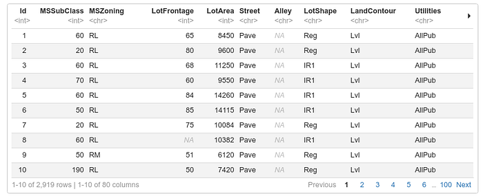
The House Price dataset, obtained from Kaggle, includes house price information. It comprises two main files: “train.csv” with 81 columns and 1460 rows, and “test.csv” with 80 columns and 1459 rows. These datasets offer extensive details on real estate properties, encompassing property type, zoning classifications, size, structural attributes, basement characteristics, interior features, heating systems, garage attributes, and more. As a valuable resource for real estate analysis and property valuation, this dataset is widely used in the field of housing market research, property appraisals, and predictive modeling to gain insights into property values and market trends, facilitating informed decision-making in the real estate industry.
Data Preprocessing
Data preprocessing is a critical step in any machine learning project, and predicting house prices with XGBoost is no exception. In this section, we’ll explore how to prepare and clean your data for effective modeling.
Loading the Dataset
# Load Library
```{r library, message=FALSE, warning=FALSE}
library(dplyr)
library(tidyr)
library(summarytools)
library(DT)
library(ggplot2)
library(printr)
library(xgboost)
library(caret)
```
# Load the Dataset
```{r data, warning=FALSE}
setwd("~/Documents/Data Task 6 & 7")
trainori <- read.csv("train.csv", header = TRUE)
testori <- read.csv("test.csv", header = TRUE)
submission <- read.csv("sample_submission.csv",header = TRUE)
sale_price <- trainori$SalePrice
train <- trainori
train <- train[,!colnames(train) %in% c("SalePrice")]
housejoin <- rbind(train,testori)
print(housejoin)
``` 
Exploratory Data Analysis (EDA)
Before diving into preprocessing, it’s essential to understand your data. EDA allows you to:
- Explore the structure of your dataset, including the number of rows and columns.
- Investigate the data types of each variable (numeric, categorical, etc.).
- Examine summary statistics to identify outliers and missing values.
```{r summary}
# Generate descriptive statistics using summarytools
desc_stats <- descr(housejoin)
desc_stats
```
Handling Missing Data
```{r check missing value}
# Define the R function to get missing value counts
get_missing_value_counts <- function(data_frame) {
  missing_counts <- colSums(is.na(data_frame))
  missing_counts <- missing_counts[missing_counts > 0]
  missing_counts <- sort(missing_counts, decreasing = TRUE)

  percent <- colSums(is.na(data_frame)) / nrow(data_frame)
  percent <- percent[percent > 0]
  percent <- sort(percent, decreasing = TRUE)

  missing_data <- data.frame(Missing_counts = missing_counts, Percent = percent)
  return(missing_data)
}

# Call the R function and print the missing value counts
train_missing_values <- get_missing_value_counts(housejoin)
print(train_missing_values)
```
Remove Column with Missing Values
```{r remove column with missing value}
# Set the threshold for missing values (70 in this example)
house_prices <- housejoin
threshold <- 70

# Calculate the number of missing values in each column
missing_values <- colSums(is.na(house_prices))

# Get the names of columns where missing values exceed the threshold >70
columns_to_remove <- names(house_prices)[missing_values > threshold]

# Remove the selected columns from the dataset
house_prices <- house_prices[, !names(house_prices) %in% columns_to_remove]
train_missing_values <- get_missing_value_counts(house_prices)
print(train_missing_values)
```
Replace Missing Value
```{r replace missing value}
# Identify character columns
char_col <- sapply(house_prices, is.character)
# Convert character columns to factors
house_prices[char_col] <- lapply(house_prices[char_col], as.factor)

# Identify factor (categorical) columns
factor_cols <- sapply(house_prices, is.factor)

# Loop through each factor column and replace missing values with the mode
for (col in names(house_prices)[factor_cols]) {
  mode_val <- names(sort(table(house_prices[[col]]), decreasing = TRUE))[1]  # Find the mode
  house_prices[is.na(house_prices[[col]]), col] <- mode_val

  # Identify integer columns
  integer_cols <- sapply(house_prices, is.integer)

  # Loop through each integer column and replace missing values with the median
  for (col in names(house_prices)[integer_cols]) {
    median_val <- median(house_prices[[col]], na.rm = TRUE)  # Calculate the median
    house_prices[[col]][is.na(house_prices[[col]])] <- median_val  # Replace missing values with the median
  }
}

print(house_prices)
```
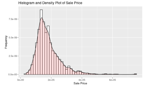
Distribution of The Data
```{r Sale Price}
ggplot(trainori, aes(x = SalePrice)) +
  geom_histogram(aes(y = after_stat(density)), binwidth = 15000, colour = "black", fill = "white") +
  geom_density(alpha = .2, fill="#FF6666") +
  ggtitle("Histogram and Density Plot of Sale Price") +
  xlab("Sale Price") + ylab("Frequency")
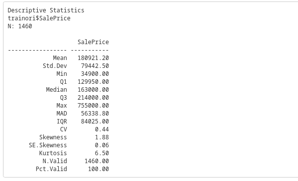
descr(trainori$SalePrice)
```
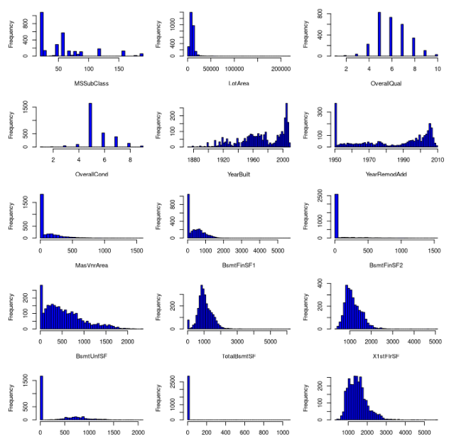
```{r hist numerical, fig.height=20, fig.width=8}
# List all the data types in the dataset
df_num <- house_prices[, !colnames(house_prices) %in% c("Id")]
data_types <- sapply(df_num, class)

# Select only the numerical features
df_num <- df_num[, data_types %in% c("numeric", "integer")]

# Set up the plot parameters for a 5x7 grid
par(mfrow=c(12, 3), mar=c(4, 4, 2, 1), oma=c(0, 0, 2, 0))

# Create histograms for each integer feature
for (i in 1:ncol(df_num)) {
  hist(df_num[, i], main="", xlab=colnames(df_num)[i], ylab="Frequency", breaks=50, col="blue")
}

# Reset plot parameters
par(mfrow=c(1, 1), mar=c(5, 4, 4, 2) + 0.1, oma=c(0, 0, 0, 0))
```
Encoding Categorical Variables
```{r dummy variable}
# Identify categorical columns in your dataset
categorical_columns <- sapply(house_prices, is.factor)

# Create dummy variables for categorical columns
data_dummies <- model.matrix(~ . - 1, data = house_prices[, categorical_columns])

# Combine the dummy variables with the numeric columns
data_processed <- cbind(house_prices[, !categorical_columns], data_dummies)

# Now, 'data_processed' contains the dataset with dummy variables for categorical columns

# You may want to rename the columns for clarity, for example:
colnames(data_processed) <- gsub("data_dummies", "", colnames(data_processed))

# Check the first few rows of the processed data
print(data_processed)
```
Train-Test Split
```{r split data}
# remove ID columns
dataset <- data_processed
dataset <- dataset[, !colnames(dataset) %in% c("Id")]
SalePrice <- sale_price

#split
datahousetrain <- cbind(dataset[1:1460,],SalePrice)

set.seed(123)  # Set a seed for reproducibility
split_ratio <- 0.7  # Adjust the ratio as needed

n <- nrow(datahousetrain)
n_train <- round(n * split_ratio)
train_inner <- datahousetrain[1:n_train, ]
test_inner <- datahousetrain[(n_train + 1):n, ]

test_actual <- dataset[1461:2919,]
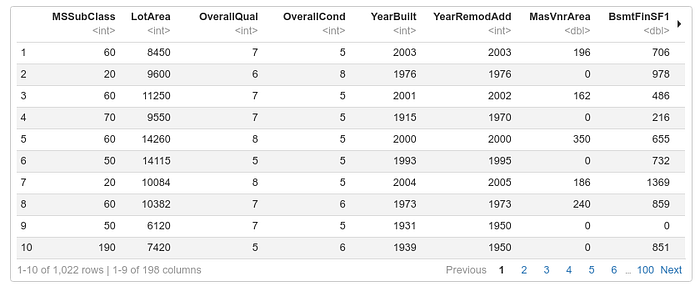
print(train_inner)
```
Building the XGBoost Model
Now that your data is prepared, it’s time to create your predictive model using XGBoost. Follow these simple steps to get started:
```{r}

x <- train_inner[,1:197]
y <- train_inner[,198]
# Never forget to exclude objective variable in 'data option'
train_Data <- xgb.DMatrix(data = as.matrix(x), label = y)

params <- list(
  objective = "reg:squarederror",
  booster = "gbtree",
  eval_metric = "rmse",
  eta = 0.3,  # Learning rate
  max_depth = 12,
  min_child_weight = 1,
  subsample = 0.8,
  colsample_bytree = 0.8
)

xgb_model <- xgboost(params = params, data = train_Data,
                     nrounds = 400, print_every_n = 100)

#1. MEAN ABSOLUTE PERCENTAGE ERROR (MAPE)
MAPE = function(y_actual,y_predict){
  mean(abs((y_actual-y_predict)/y_actual))*100
}

#2. R SQUARED error metric -- Coefficient of Determination
RSQUARE = function(y_actual,y_predict){
  cor(y_actual,y_predict)^2
}

train_pred <- predict(xgb_model,train_Data)
rmse_train <- RMSE(y,train_pred)
r2_train <- RSQUARE(y,train_pred)
mape_train <- MAPE(y,train_pred)

namesmetrictrain <- c("RMSE Train","R Squared Train","MAPE Train")
scoremetrictrain <- c(rmse_train,r2_train,mape_train)
resultstrain<- as.data.frame(cbind(namesmetrictrain,scoremetrictrain))
colnames(resultstrain) <- c("Results","Score")
print(resultstrain)

```

```{r importance}
# Get feature importance scores
importance_matrix <- xgb.importance(model = xgb_model)

# Create Bar chart
xgb.plot.importance(importance_matrix[1:10,])
```
```{r}
x_test <- test_inner[,1:197]
y_test <- test_inner[,198]
test_Data <- xgb.DMatrix(data = as.matrix(x_test))
test_pred <- predict(xgb_model,test_Data)
rmse_test <- RMSE(y_test,test_pred)
r2_test <- RSQUARE(y_test,test_pred)
mape_test <- MAPE(y_test,test_pred)

namesmetrictest <- c("RMSE Test","R Squared Test","MAPE Test")
scoremetrictest<- c(rmse_test,r2_test,mape_test)
resultstest <- as.data.frame(cbind(namesmetrictest,scoremetrictest))
colnames(resultstest) <- c("Results","Score")
print(resultstest)
``````{r}

x_test <- test_inner[,1:197]
y_test <- test_inner[,198]
test_Data <- xgb.DMatrix(data = as.matrix(x_test))
test_pred <- predict(xgb_model,test_Data)
rmse_test <- RMSE(y_test,test_pred)
r2_test <- RSQUARE(y_test,test_pred)
mape_test <- MAPE(y_test,test_pred)

namesmetrictest <- c("RMSE Test","R Squared Test","MAPE Test")
scoremetrictest<- c(rmse_test,r2_test,mape_test)
resultstest <- as.data.frame(cbind(namesmetrictest,scoremetrictest))
colnames(resultstest) <- c("Results","Score")
print(resultstest)
```
```{r}
testactual_xgb <- xgb.DMatrix(data = as.matrix(test_actual))
pred_testactual <- predict(xgb_model,testactual_xgb)
submission_xgb <- as.data.frame(cbind(submission$Id,pred_testactual))
colnames(submission_xgb) <- c("Id","PredictedSalePrice")
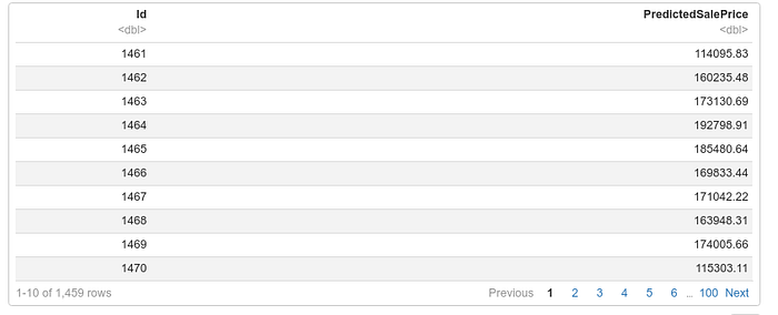
print(submission_xgb)

```